How Dijkstra’s Algorithm Works with Visual Example
In this article, I’m gonna explain how Dijsktra’s algorithm works, so that you can use it to build some cool stuff :)
Here’s a visual example of Dijsktra’s algorithm.

General
Dijkstra’s algorithm is a graph-searching algorithm that’s used to find the shortest path between two nodes in a graph. The algorithm is used — or serves as a basis — in areas such as telecommunications, maze-solving, and navigation systems.
The only requirement for the algorithm to run is to
- Represent the system as a graph
- Know the start and the end nodes
The classic example is using Maps. In the image, the start node is A, and the end node is B.
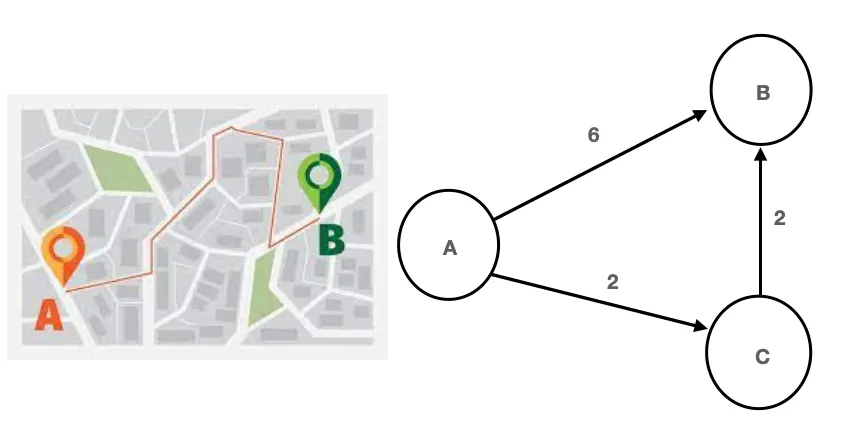
Nodes are intersections (A, B, and C), and edges are roads connecting any two nodes. Each edge has a certain cost attributed to it — also known as weight. If a road is more crowded, it has a higher weight and vice versa.
From the map example, you would say:
“The shortest time to get from A to B is 4 minutes.”
Visual explanation
How it works
In short, the algorithm keeps track of all node’s distances from the start node. The algorithm starts from the start node, and it does these two steps over, and over again.
- Expands on the node with the current shortest distance from the start
- Updates the distances from the start node
Once “the node with the shortest distance from the start” becomes the end node, you found the shortest path! :)
Explanation setup
Let’s say you have a map represented as a 2D array of squares.

Each square represents a node, and each node is connected to any of its neighbors. This means that each node can have up to 8 neighboring nodes.

In this environment, let's say that the cost to move vertically or horizontally is 1, and to move to any diagonal neighbor is 2 (just like the time to go through a road, in the example before).

The costs of the paths are set this way as an example, so the diagonal movement costs more. But, these numbers are just an example; They can be anything.
Algorithm
Here is the step-by-step walkthrough.
Throughout the algorithm, use a priority queue to keep track of all nodes you visited.
visited = []
Firstly, you should
- Define the start (play button) and end (flag) nodes
- Set the “distance from the start node” for all nodes to infinity.

Start from the start node, set its distance to 0, and add it to the priority queue.
visited = [0]
Pop the first node in the queue, and mark it as done (marked blue).
visited = []

Then, visit all the neighboring nodes of the node you just popped. The neighbors are highlighted below.

For each neighbor you visit, if not already marked as done, do:
- Calculate the distance to go to that neighbor
- If the distance is shorter than the currently set one, update the shortest distance to go to the neighbour
- If you update it, add it to the priority queue
First iteration
Each step, starting from the top left neighbour, is as follows.

The current shortest distance to reach the top left neighbour is set to infinity. If you travel from the current node to the neighbour, what distance would that be?
New distance = distance to current node(0) + distance to go to neighbour(2)
Is the new distance smaller than the current one (2 < infinity)? — Yes!
Therefore,
- Update the current shortest distance to go to the neighbouring node
- Add the neighbour to the queue
- Go to the next neighbour
visited = [2]

For the next neighbour,
New distance = 0 + 1
Is 1< infinity? — Yes! Then,
- Update the current shortest distance to the neighbouring node
- Add the neighbour to the queue
- Go to the next neighbour
visited = [2, 1]

Repeat for all neighbours…
visited = [2, 1, 2, 1, 1, 2, 1, 2]

After visiting all nodes, you sort the queue so the node with the shortest distance to reach is at the end of the queue.
visited = [1, 1, 1, 1, 2, 2, 2, 2]

Colors indicate:
- Orange, nodes in the queue
- Blue, all the done nodes (popped from the queue)
- Green, the current node with the lowest distance from the start (first in the queue)
Second iteration
Then, repeat the same steps again.
- Pop the first node from the queue (node marked with green)
- Visit all its neighbours, who are not marked as done

For the first top left neighbour,
New distance = 1 (shortest distance to the current node) + 2 (distance to move diagonally)
Is 2 < 1? — NO! This means that path to this neighbouring node, through the current node, isn’t the shortest path to the neighbouring node. And, indeed, the shortest one is from the start node, and then up.
visited = [1, 1, 1, 2, 2, 2, 2]

The next neighbour is the start node. It’s marked as done (blue), which means it’s already been popped from the queue, and you can skip it.
Next is the bottom left neighbour,
New distance = 1 + 2
Is 2 < 1? — NO! Don’t do anything, go to the next neighbour.
visited = [1, 1, 1, 2, 2, 2, 2]

For the top neighbour,
New distance = 1 + 1(distance to move vertical or horizontal)
Is 2 < 2? — NO! Don’t do anything, go to the next neighbour.
visited = [1, 1, 1, 2, 2, 2, 2]

For the bottom neighbour, same thing,
New distance = 1 + 1
Is 2 < 2? — NO! Don’t do anything, go to the next neighbour.
visited = [1, 1, 1, 2, 2, 2, 2]

For the top right neighbour,
New distance = 1 + 2
Is 3 < Infinity? — YES! Therefore,
- Update the shortest distance to the node
- Add it to the queue
…
I think you get the algorithm by now. Here is what the second iteration looks like in motion.
visited = [1, 1, 1, 2, 2, 2, 2, 3, 2, 3]

At the end of the iteration, you again sort the queue. This is the final position after the second iteration.
visited = [1, 1, 1, 2, 2, 2, 2, 2, 3, 3]

Iterations loop over until either
- The popped node is the goal node — you found the shortest path :)
- The queue is empty — there is no path to the goal node
Seeing the algorithm in action looks like this,

It's right there?!
As you can see from the GIF above, Dijkstra’s algorithm lacks a sense of direction. It expands in all directions, unaware of where the goal node is. This behaviour can make the algorithm look silly when the end is next to it, like in the GIF above.
A* algorithm expands on Dijkstra by adding another criterion for expanding — distance from the goal node.
Play around with the algorithms
Check out my playground visualization of path-finding algorithms made with Flutter. It enables you to visualize A* too :)
Feel free to take a look at the source code for the algorithm implementation.
If you have any questions feel free to leave a comment or contact me on twitter.
See you 👋